Using BERT to predict disaster Tweets
In 2019, Kaggle hosted the Natural Language Processing with Disaster Tweets competition. It was made for contestants to test their ability to build a machine learning model able to understand the nuances of natural language and able to predict whether a tweet is about a real disaster or not. Today, this contest is one of Kaggle’s most popular competitions used to learn about NLP and test the capabilities of various language models.
In this notebook, we are going to build two deep learning solutions based on BERT in order to predict the tweets.
import torch
import base64
import random
import numpy as np
import pandas as pd
from torch import nn
from tqdm.auto import tqdm
from rich.table import Table
from torchinfo import summary
from rich.console import Console
from torch.utils.data import Dataset
from IPython.display import Image, display
from transformers import BertModel, BertTokenizer, get_scheduler
from sklearn.metrics import f1_score, accuracy_score, precision_score, recall_score, roc_auc_score

torch.manual_seed(0)
random.seed(0)
np.random.seed(0)
console = Console()
About the data
Kaggle provides us with a dataset containing tweets and a binary label indicating whether this data is about a real disaster or not. The data contains three predictors: text, keyword, and location.
We will start by creating helper functions to load both the train and test data.
FULL_TRAIN_DATA_PATH = '/kaggle/input/nlp-getting-started/train.csv'
TEST_DATA_PATH = '/kaggle/input/nlp-getting-started/test.csv'

def load_full_raw_train_df():
    return pd.read_csv(FULL_TRAIN_DATA_PATH)

def load_raw_test_df():
    return pd.read_csv(TEST_DATA_PATH)

def rich_display_dataframe(df, title="Dataframe", style = None):
    df = df.astype(str)
    table = Table(title=title)
    for i, col in enumerate(df.columns):
        if style is None:
            table.add_column(col)
        else:
            table.add_column(col, style=style[i])
    for row in df.values:
        table.add_row(*row)
    console.print(table)

full_train_df = load_full_raw_train_df()

rich_display_dataframe(full_train_df.head(), title="Full-Train Dataframe")
Full-Train Dataframe ┏━━━━┳━━━━━━━━━┳━━━━━━━━━━┳━━━━━━━━━━━━━━━━━━━━━━━━━━━━━━━━━━━━━━━━━━━━━━━━━━━━━━━━━━━━━━━━━━━━━━━━━━━━━━┳━━━━━━━━┓ ┃ id ┃ keyword ┃ location ┃ text ┃ target ┃ ┡━━━━╇━━━━━━━━━╇━━━━━━━━━━╇━━━━━━━━━━━━━━━━━━━━━━━━━━━━━━━━━━━━━━━━━━━━━━━━━━━━━━━━━━━━━━━━━━━━━━━━━━━━━━╇━━━━━━━━┩ │ 1 │ nan │ nan │ Our Deeds are the Reason of this #earthquake May ALLAH Forgive us all │ 1 │ │ 4 │ nan │ nan │ Forest fire near La Ronge Sask. Canada │ 1 │ │ 5 │ nan │ nan │ All residents asked to 'shelter in place' are being notified by officers. No │ 1 │ │ │ │ │ other evacuation or shelter in place orders are expected │ │ │ 6 │ nan │ nan │ 13,000 people receive #wildfires evacuation orders in California │ 1 │ │ 7 │ nan │ nan │ Just got sent this photo from Ruby #Alaska as smoke from #wildfires pours │ 1 │ │ │ │ │ into a school │ │ └────┴─────────┴──────────┴──────────────────────────────────────────────────────────────────────────────┴────────┘
While building the model, we would like to know how well our model is performing. To do that, we are going to use a validation dataset to check our model’s predictions.
TRAIN_DATA_RATIO = 0.9
TRAIN_DATA_PATH = './train.csv'
VAL_DATA_PATH = './val.csv'

def create_train_val_split():
    df = load_full_raw_train_df()
    train_no_samples = round(TRAIN_DATA_RATIO * df.shape[0])
    train = df.sample(train_no_samples)
    val = df.drop(train.index)
    train.to_csv(TRAIN_DATA_PATH, index=False)
    val.to_csv(VAL_DATA_PATH, index=False)

create_train_val_split()

def load_raw_train_df():
    return pd.read_csv(TRAIN_DATA_PATH)

def load_raw_val_df():
    return pd.read_csv(VAL_DATA_PATH)

train_df = load_raw_train_df()
val_df = load_raw_val_df()

rich_display_dataframe(train_df.head(), title="Train Dataframe")
Train Dataframe ┏━━━━━━┳━━━━━━━━━━━━━━━━┳━━━━━━━━━━━━━━━━━━━━━━━━━━━┳━━━━━━━━━━━━━━━━━━━━━━━━━━━━━━━━━━━━━━━━━━━━━━━━━━━━┳━━━━━━━━┓ ┃ id ┃ keyword ┃ location ┃ text ┃ target ┃ ┡━━━━━━╇━━━━━━━━━━━━━━━━╇━━━━━━━━━━━━━━━━━━━━━━━━━━━╇━━━━━━━━━━━━━━━━━━━━━━━━━━━━━━━━━━━━━━━━━━━━━━━━━━━━╇━━━━━━━━┩ │ 454 │ armageddon │ Wrigley Field │ @KatieKatCubs you already know how this shit goes. │ 0 │ │ │ │ │ World Series or Armageddon. │ │ │ 7086 │ meltdown │ Two Up Two Down │ @LeMaireLee @danharmon People Near Meltdown Comics │ 0 │ │ │ │ │ Who Have Free Time to Wait in Line on Sunday │ │ │ │ │ │ Nights are not a representative sample. #140 │ │ │ 762 │ avalanche │ Score Team Goals Buying @ │ 1-6 TIX Calgary Flames vs COL Avalanche Preseason │ 0 │ │ │ │ │ 9/29 Scotiabank Saddledome http://t.co/5G8qA6mPxm │ │ │ 9094 │ suicide%20bomb │ Roadside │ If you ever think you running out of choices in │ 0 │ │ │ │ │ life rembr there's that kid that has no choice but │ │ │ │ │ │ wear a suicide bomb vest │ │ │ 1160 │ blight │ Laventillemoorings │ If you dotish to blight your car go right ahead. │ 0 │ │ │ │ │ Once it's not mine. │ │ └──────┴────────────────┴───────────────────────────┴────────────────────────────────────────────────────┴────────┘
Metaphor’s Misuse
A challenge facing our model is the figurative use of tragedy related terms. For example, consider the following two Tweets.
table = Table(title="Confusion Caused by Figurative Use of Words")
table.add_column("Tweet", style='blue')
table.add_column("Is Related to Disaster?", style='red', justify='center')

table.add_row(train_df.iloc[677]['text'], 'Disaster' if train_df.iloc[677]['target'] == 1 else 'Not a Disaster')
table.add_row(train_df.iloc[6170]['text'], 'Disaster' if train_df.iloc[6170]['target'] == 1 else 'Not a Disaster')

console.print(table)
Confusion Caused by Figurative Use of Words ┏━━━━━━━━━━━━━━━━━━━━━━━━━━━━━━━━━━━━━━━━━━━━━━━━━━━━━━━━━━━━━━━━━━━━━━━━━━━━━━┳━━━━━━━━━━━━━━━━━━━━━━━━━┓ ┃ Tweet ┃ Is Related to Disaster? ┃ ┡━━━━━━━━━━━━━━━━━━━━━━━━━━━━━━━━━━━━━━━━━━━━━━━━━━━━━━━━━━━━━━━━━━━━━━━━━━━━━━╇━━━━━━━━━━━━━━━━━━━━━━━━━┩ │ @bbcmtd Wholesale Markets ablaze http://t.co/lHYXEOHY6C │ Disaster │ │ On plus side LOOK AT THE SKY LAST NIGHT IT WAS ABLAZE http://t.co/qqsmshaJ3N │ Not a Disaster │ └──────────────────────────────────────────────────────────────────────────────┴─────────────────────────┘
Although both Tweets share the term ablaze, they mean very different things. In the first sentence ablaze is used to mean burning fiercely, and in the second sentence it means brightly coloured or lighted. Thus, the context of the words specify its meaning, thus, determining its classification.
We learn from this that in order to reach high accuracy, we need to use a model that is able to understand the full context of the sentence. We expect model’s like CountVictorizer to fail due to their inability to understand the nuances of language and the context of the terms.
Proposed Model
In order to understand the context of the sentence, we are going to use a pretrained language model. This model is able to generate an embedding vector from given text. This embedding is a high dimensional vector having the property that the closer the embeddings are to each other the more semantically similar are the text inputs. Such model gives us the ability to understand the intended meaning of the tweets.
After generating the embeddings, we are going to use a small classification head to make our predictions. This head is a small deep learning model that we are going to train. It takes the embeddings as input and generate the final prediction.
Here is a diagram showing a high level overview of the model.
def mm(graph):
    graph_bytes = graph.encode("utf8")
    base64_bytes = base64.urlsafe_b64encode(graph_bytes)
    base64_string = base64_bytes.decode("ascii")
    display(Image(url="https://mermaid.ink/img/" + base64_string))

mm("""
flowchart LR
    data[Tweet]
    model[Pretrained Language Model]
    head[Binary Classification Head]
    output[Prediction]
    data --> model --> head --> output
""")
The Pretrained Language Model
The pretrained language model we are going to use is BERT. BERT, Bidirectional Encoder Representations from Transformers, is an open-source language representation model developed by researchers at Google in October 2018. It was trained on a large corpus including the Toronto Book Corpus and Wikipedia.
There are two important versions of the model: bert-base and bert-large. The difference is in the size of the model and the size of the embeddings vector. As indicated by its name, bert-large is nearly 3 times larger than bret-base. While its size helps it be more accurate, it makes it slower and more expensive to use. Thus, we will start by using the bert-base version.
The following shows the model architecture.
bert = BertModel.from_pretrained('google-bert/bert-base-uncased')
summary(bert)
config.json: 0%| | 0.00/570 [00:00<?, ?B/s]
model.safetensors: 0%| | 0.00/440M [00:00<?, ?B/s]
================================================================================
Layer (type:depth-idx) Param #
================================================================================
BertModel --
├─BertEmbeddings: 1-1 --
│ └─Embedding: 2-1 23,440,896
│ └─Embedding: 2-2 393,216
│ └─Embedding: 2-3 1,536
│ └─LayerNorm: 2-4 1,536
│ └─Dropout: 2-5 --
├─BertEncoder: 1-2 --
│ └─ModuleList: 2-6 --
│ │ └─BertLayer: 3-1 7,087,872
│ │ └─BertLayer: 3-2 7,087,872
│ │ └─BertLayer: 3-3 7,087,872
│ │ └─BertLayer: 3-4 7,087,872
│ │ └─BertLayer: 3-5 7,087,872
│ │ └─BertLayer: 3-6 7,087,872
│ │ └─BertLayer: 3-7 7,087,872
│ │ └─BertLayer: 3-8 7,087,872
│ │ └─BertLayer: 3-9 7,087,872
│ │ └─BertLayer: 3-10 7,087,872
│ │ └─BertLayer: 3-11 7,087,872
│ │ └─BertLayer: 3-12 7,087,872
├─BertPooler: 1-3 --
│ └─Linear: 2-7 590,592
│ └─Tanh: 2-8 --
================================================================================
Total params: 109,482,240
Trainable params: 109,482,240
Non-trainable params: 0
================================================================================Building the Model
Now we are going to use PyTorch to add the classification head to bert.
class Model(nn.Module):
    def __init__(self):
        super().__init__()
        self.bert = BertModel.from_pretrained('google-bert/bert-base-uncased')
        self.head = nn.Sequential(nn.LazyLinear(2))

    def forward(self, input_ids: torch.Tensor,
                attention_mask: torch.Tensor,
                labels: torch.Tensor = None):
        outputs = self.bert(input_ids=input_ids, attention_mask=attention_mask)
        hidden_layer = outputs['pooler_output']

        logits = self.head(hidden_layer)

        if labels is not None:
            loss = nn.functional.cross_entropy(logits, labels)
            return {'loss': loss, 'logits': logits}
        else:
            return {'logits': logits}

model = Model()

summary(model)
=====================================================================================
Layer (type:depth-idx) Param #
=====================================================================================
Model --
├─BertModel: 1-1 --
│ └─BertEmbeddings: 2-1 --
│ │ └─Embedding: 3-1 23,440,896
│ │ └─Embedding: 3-2 393,216
│ │ └─Embedding: 3-3 1,536
│ │ └─LayerNorm: 3-4 1,536
│ │ └─Dropout: 3-5 --
│ └─BertEncoder: 2-2 --
│ │ └─ModuleList: 3-6 85,054,464
│ └─BertPooler: 2-3 --
│ │ └─Linear: 3-7 590,592
│ │ └─Tanh: 3-8 --
├─Sequential: 1-2 --
│ └─LazyLinear: 2-4 --
=====================================================================================
Total params: 109,482,240
Trainable params: 109,482,240
Non-trainable params: 0
=====================================================================================We are now ready to start training the model. This training process is responsible for training the classification head from scratch and fine-tuning the BERT model on the data making it more accurate to our use case.
class KeyedDataset(Dataset):
    def __init__(self, **tensor_dict):
        self.tensor_dict = tensor_dict

        for key, tensor in tensor_dict.items():
            assert isinstance(tensor, torch.Tensor)
            assert tensor.size(0) == tensor_dict[next(iter(tensor_dict))].size(0)

    def __len__(self):
        return next(iter(self.tensor_dict.values())).size(0)

    def __getitem__(self, idx):
        return {key: tensor[idx] for key, tensor in self.tensor_dict.items()}

def create_dataset(df: pd.DataFrame, include_labels=True) -> KeyedDataset:
    tokenizer = BertTokenizer.from_pretrained('google-bert/bert-base-uncased', do_lower_case=True)
    encoded_dict = tokenizer(df['text'].tolist(), padding=True, truncation=True, return_tensors='pt')
    input_ids = encoded_dict['input_ids']
    attention_mask = encoded_dict['attention_mask']

    if include_labels:
        labels = torch.tensor(df['target'].tolist())
        return KeyedDataset(input_ids=input_ids,
                            attention_mask=attention_mask,
                            labels=labels)
    else:
        return KeyedDataset(input_ids=input_ids,
                            attention_mask=attention_mask)

def train(model: nn.Module,
          train_dataloader: torch.utils.data.DataLoader,
          eval_dataloader: torch.utils.data.DataLoader = None,
          device: torch.device = torch.device('cpu'),
          lr: float = 5e-5,
          epochs: int = 4):
    model = model.to(device)
    optimizer = torch.optim.AdamW(model.parameters(), lr=lr)
    num_training_steps = len(train_dataloader) * epochs
    lr_scheduler = get_scheduler('linear', optimizer, num_warmup_steps=0, num_training_steps=num_training_steps)
    progress = tqdm(range(num_training_steps))

    table = Table()
    table.add_column('Metric')
    table.add_column('f1', style='red')
    table.add_column('Accuracy')
    table.add_column('Precision')
    table.add_column('Recall')
    table.add_column('roc_auc')

    for epoch in range(epochs):
        model.train()
        for batch in train_dataloader:
            batch = {key: value.to(device) for key, value in batch.items()}
            outputs = model(**batch)
            loss = outputs['loss']
            loss.backward()
            optimizer.step()
            lr_scheduler.step()
            optimizer.zero_grad()
            progress.update()
            progress.set_postfix({'loss': loss.item()})

        model.eval()
        predictions_list = []
        labels_list = []
        with torch.no_grad():
            for batch in eval_dataloader:
                batch = {key: value.to(device) for key, value in batch.items()}
                outputs = model(**batch)
                predictions = outputs['logits'].argmax(dim=1)
                predictions_list.extend(predictions.tolist())
                labels_list.extend(batch['labels'].tolist())
        table.add_row(f'Epoch: {epoch+1}',
            f"{round(f1_score(labels_list, predictions_list) * 100, 3)}%",
            f"{round(accuracy_score(labels_list, predictions_list) * 100, 3)}%",
            f"{round(precision_score(labels_list, predictions_list) * 100, 3)}%",
            f"{round(recall_score(labels_list, predictions_list) * 100, 3)}%",
            f"{round(roc_auc_score(labels_list, predictions_list) * 100, 3)}%")
    console.print(table)


train_df = load_raw_train_df()
val_df = load_raw_val_df()

train_dataset = create_dataset(train_df)
val_dataset = create_dataset(val_df)

train_dataloader = torch.utils.data.DataLoader(train_dataset, batch_size=32, shuffle=True)
val_dataloader = torch.utils.data.DataLoader(val_dataset, batch_size=32, shuffle=False)

device = torch.device('cpu')

if torch.backends.mps.is_available():
    device = torch.device('mps')
elif torch.cuda.is_available():
    device = torch.device('cuda')

model = Model()
tokenizer_config.json: 0%| | 0.00/48.0 [00:00<?, ?B/s]
vocab.txt: 0%| | 0.00/232k [00:00<?, ?B/s]
tokenizer.json: 0%| | 0.00/466k [00:00<?, ?B/s]train(model=model,
train_dataloader=train_dataloader,
eval_dataloader=val_dataloader,
device=device,
lr=5e-5,
epochs=4) 0%| | 0/860 [00:00<?, ?it/s]┏━━━━━━━━━━┳━━━━━━━━━┳━━━━━━━━━━┳━━━━━━━━━━━┳━━━━━━━━━┳━━━━━━━━━┓ ┃ Metric ┃ f1 ┃ Accuracy ┃ Precision ┃ Recall ┃ roc_auc ┃ ┡━━━━━━━━━━╇━━━━━━━━━╇━━━━━━━━━━╇━━━━━━━━━━━╇━━━━━━━━━╇━━━━━━━━━┩ │ Epoch: 1 │ 77.465% │ 83.18% │ 90.164% │ 67.901% │ 81.205% │ │ Epoch: 2 │ 78.827% │ 82.917% │ 83.448% │ 74.691% │ 81.854% │ │ Epoch: 3 │ 78.146% │ 82.654% │ 84.286% │ 72.84% │ 81.385% │ │ Epoch: 4 │ 78.438% │ 81.866% │ 79.43% │ 77.469% │ 81.297% │ └──────────┴─────────┴──────────┴───────────┴─────────┴─────────┘
Utilizing the Keywords
Now, we have successfully built a model that is able to do the prediction, and we can submit it to the competition. However, we are going to build another model to further increase our performance.
The keyword field seems promising. It’s my belief that this field will help the model make its classification. But how can we use the data to check our hypothesis?
The best possible model for classifying tweets using only the keyword is a Bayes classifier which works by calculating P( Tweet Refers to Disaster | Keyword ) Before we start building a model, we can get a feel for the validity of the hypothesis by calculating P( Tweet Refers to Disaster | Keyword ) for each of the keywords in the training dataset. If the range of probabilities is wide, then our hypothesis is correct, and we are going to build a model that extrapolates to unseen keywords.
def create_keywords_stats_df(df: pd.DataFrame):
    keywords = df['keyword'][~df['keyword'].isna()].unique()
    prob_disaster_given_keyword_list = []
    no_tweets_list = []
    for keyword in keywords:
        prob_disaster_given_keyword = ((df['target']==1) & (df['keyword']==keyword)).sum() / (df['keyword']==keyword).sum()
        no_tweets = (df['keyword']==keyword).sum()
        prob_disaster_given_keyword_list.append(prob_disaster_given_keyword)
        no_tweets_list.append(no_tweets)
    keyword_stats_df = pd.DataFrame({
        'Keyword': keywords,
        'P(Tweet Refers to Disaster | Keyword)': prob_disaster_given_keyword_list,
        'No. Tweets': no_tweets_list
    })
    keyword_stats_df['Keyword'] = keyword_stats_df['Keyword'].str.replace('%20', ' ')
    return keyword_stats_df

keyword_stats_df = create_keywords_stats_df(train_df)
keyword_stats_df = keyword_stats_df.sort_values('P(Tweet Refers to Disaster | Keyword)')

keyword_stats_df['P(Tweet Refers to Disaster | Keyword)'] = keyword_stats_df['P(Tweet Refers to Disaster | Keyword)'].apply(
    lambda x: f"{round(100 * x, 3)}%")

rich_display_dataframe(keyword_stats_df.head(15),
                       style = ['blue', 'red', 'green'],
                       title = 'Keyword with Lowest Disaster Probability')

rich_display_dataframe(keyword_stats_df.iloc[::-1].head(15),
                       style = ['blue', 'red', 'green'],
                       title = 'Keyword with Highest Disaster Probability')
Keyword with Lowest Disaster Probability ┏━━━━━━━━━━━━━┳━━━━━━━━━━━━━━━━━━━━━━━━━━━━━━━━━━━━━━━┳━━━━━━━━━━━━┓ ┃ Keyword ┃ P(Tweet Refers to Disaster | Keyword) ┃ No. Tweets ┃ ┡━━━━━━━━━━━━━╇━━━━━━━━━━━━━━━━━━━━━━━━━━━━━━━━━━━━━━━╇━━━━━━━━━━━━┩ │ aftershock │ 0.0% │ 32 │ │ body bags │ 2.778% │ 36 │ │ ruin │ 3.03% │ 33 │ │ screaming │ 3.03% │ 33 │ │ blazing │ 3.333% │ 30 │ │ electrocute │ 3.333% │ 30 │ │ body bag │ 3.448% │ 29 │ │ traumatised │ 6.061% │ 33 │ │ panic │ 6.061% │ 33 │ │ wrecked │ 6.25% │ 32 │ │ bloody │ 6.452% │ 31 │ │ blew up │ 6.667% │ 30 │ │ blight │ 7.143% │ 28 │ │ panicking │ 7.407% │ 27 │ │ obliterated │ 7.692% │ 26 │ └─────────────┴───────────────────────────────────────┴────────────┘
                Keyword with Highest Disaster Probability
┏━━━━━━━━━━━━━━━━━━┳━━━━━━━━━━━━━━━━━━━━━━━━━━━━━━━━━━━━━━━┳━━━━━━━━━━━━┓
┃ Keyword          ┃ P(Tweet Refers to Disaster | Keyword) ┃ No. Tweets ┃
┡━━━━━━━━━━━━━━━━━━╇━━━━━━━━━━━━━━━━━━━━━━━━━━━━━━━━━━━━━━━╇━━━━━━━━━━━━┩
│ wreckage         │ 100.0%                                │ 34         │
│ derailment       │ 100.0%                                │ 36         │
│ debris           │ 100.0%                                │ 31         │
│ outbreak         │ 97.222%                               │ 36         │
│ typhoon          │ 96.97%                                │ 33         │
│ oil spill        │ 96.875%                               │ 32         │
│ rescuers         │ 96.875%                               │ 32         │
│ suicide bomber   │ 96.774%                               │ 31         │
│ suicide bombing  │ 96.552%                               │ 29         │
│ nuclear disaster │ 93.103%                               │ 29         │
│ bombing          │ 92.0%                                 │ 25         │
│ suicide bomb     │ 90.909%                               │ 33         │
│ wildfire         │ 89.655%                               │ 29         │
│ evacuated        │ 88.235%                               │ 34         │
│ razed            │ 87.879%                               │ 33         │
└──────────────────┴───────────────────────────────────────┴────────────┘
We can see that the probabilities have a wide range which suggest to us to move further with our new idea.
The Updated Model
This time we are going to embed both the keywords and the Tweet, concatenate the embeddings, and then pass the new vector to a classification head.
mm("""
flowchart LR
    data[Tweet]
    model1[Pretrained Language Model]
    model2[Pretrained Language Model]
    keyword[Keyword]
    head[Binary Classification Head]
    output[Prediction]
    data --> model1 --> head --> output
    keyword --> model2 --> head
""")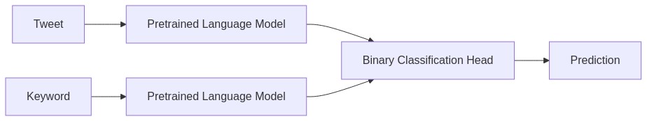
We are going to use bert-large for the text and bert-base for the keywords.
class Model(nn.Module):
    def __init__(self):
        super().__init__()
        self.text_bert = BertModel.from_pretrained('google-bert/bert-large-uncased')
        self.text_bert_no_hidden = 1024

        self.keyword_bert = BertModel.from_pretrained('google-bert/bert-base-uncased')
        self.keyword_bert_no_hidden = 768

        self.head = nn.Sequential(nn.LazyLinear(512),
                                  nn.ReLU(),
                                  nn.LazyLinear(2))

    def forward(self, text_input_ids: torch.Tensor,
                text_attention_mask: torch.Tensor,
                keyword_input_ids: torch.Tensor,
                keyword_attention_mask: torch.Tensor,
                labels: torch.Tensor = None):
        text_outputs = self.text_bert(input_ids=text_input_ids, attention_mask=text_attention_mask)
        text_hidden_layer = text_outputs['pooler_output']

        keyword_outputs = self.keyword_bert(input_ids=keyword_input_ids, attention_mask=keyword_attention_mask)
        keyword_hidden_layer = keyword_outputs['pooler_output']

        full_hidden_layer = torch.cat((text_hidden_layer, keyword_hidden_layer), dim=1)

        logits = self.head(full_hidden_layer)

        if labels is not None:
            loss = nn.functional.cross_entropy(logits, labels)
            return {'loss': loss, 'logits': logits}
        else:
            return {'logits': logits}

def create_dataset(df: pd.DataFrame, include_labels=True) -> KeyedDataset:
    df['keyword'] = df['keyword'].fillna('')

    tokenizer = BertTokenizer.from_pretrained('google-bert/bert-large-uncased', do_lower_case=True)
    encoded_dict = tokenizer(df['text'].tolist(), padding=True, truncation=True, return_tensors='pt')
    text_input_ids = encoded_dict['input_ids']
    text_attention_mask = encoded_dict['attention_mask']

    tokenizer = BertTokenizer.from_pretrained('google-bert/bert-base-uncased', do_lower_case=True)
    encoded_dict = tokenizer(df['keyword'].tolist(), padding=True, truncation=True, return_tensors='pt')
    keyword_input_ids = encoded_dict['input_ids']
    keyword_attention_mask = encoded_dict['attention_mask']

    if include_labels:
        labels = torch.tensor(df['target'].tolist())
        return KeyedDataset(text_input_ids=text_input_ids,
                            text_attention_mask=text_attention_mask,
                            keyword_input_ids=keyword_input_ids,
                            keyword_attention_mask=keyword_attention_mask,
                            labels=labels)
    else:
        return KeyedDataset(text_input_ids=text_input_ids,
                            text_attention_mask=text_attention_mask,
                            keyword_input_ids=keyword_input_ids,
                            keyword_attention_mask=keyword_attention_mask)
train_df = load_raw_train_df()
val_df = load_raw_val_df()
train_dataset = create_dataset(train_df)
val_dataset = create_dataset(val_df)
train_dataloader = torch.utils.data.DataLoader(train_dataset, batch_size=32, shuffle=True)
val_dataloader = torch.utils.data.DataLoader(val_dataset, batch_size=32, shuffle=False)
model = Model()tokenizer_config.json: 0%| | 0.00/48.0 [00:00<?, ?B/s]
vocab.txt: 0%| | 0.00/232k [00:00<?, ?B/s]
tokenizer.json: 0%| | 0.00/466k [00:00<?, ?B/s]
config.json: 0%| | 0.00/571 [00:00<?, ?B/s]
model.safetensors: 0%| | 0.00/1.34G [00:00<?, ?B/s]train(model=model,
train_dataloader=train_dataloader,
eval_dataloader=val_dataloader,
device=device,
lr=5e-5,
epochs=4) 0%| | 0/860 [00:00<?, ?it/s]┏━━━━━━━━━━┳━━━━━━━━━┳━━━━━━━━━━┳━━━━━━━━━━━┳━━━━━━━━━┳━━━━━━━━━┓ ┃ Metric ┃ f1 ┃ Accuracy ┃ Precision ┃ Recall ┃ roc_auc ┃ ┡━━━━━━━━━━╇━━━━━━━━━╇━━━━━━━━━━╇━━━━━━━━━━━╇━━━━━━━━━╇━━━━━━━━━┩ │ Epoch: 1 │ 80.569% │ 83.837% │ 82.524% │ 78.704% │ 83.173% │ │ Epoch: 2 │ 79.263% │ 82.26% │ 78.899% │ 79.63% │ 81.92% │ │ Epoch: 3 │ 78.425% │ 81.997% │ 80.064% │ 76.852% │ 81.332% │ │ Epoch: 4 │ 79.805% │ 83.706% │ 84.483% │ 75.617% │ 82.66% │ └──────────┴─────────┴──────────┴───────────┴─────────┴─────────┘
def predict(model: nn.Module,
            dataloader: torch.utils.data.DataLoader,
            device = torch.device('cpu')):
    predictions = []
    model.to(device)
    model.eval()
    with torch.no_grad():
        for batch in dataloader:
            batch = {key: val.to(device) for key, val in batch.items()}
            outputs = model(**batch)
            predictions.extend(outputs['logits'].argmax(dim=1).tolist())
    return predictions

test_df = load_raw_test_df()
test_dataset = create_dataset(test_df, include_labels=False)
test_dataloader = torch.utils.data.DataLoader(test_dataset, batch_size=32, shuffle=False)

test_df['target'] = predict(model, test_dataloader, device)
test_df = test_df[['id', 'target']]
rich_display_dataframe(test_df.head(10), title = 'Test Predictions')
test_df.to_csv('submission.csv', index=False)
Test Predictions ┏━━━━┳━━━━━━━━┓ ┃ id ┃ target ┃ ┡━━━━╇━━━━━━━━┩ │ 0 │ 1 │ │ 2 │ 1 │ │ 3 │ 1 │ │ 9 │ 1 │ │ 11 │ 1 │ │ 12 │ 1 │ │ 21 │ 0 │ │ 22 │ 0 │ │ 27 │ 0 │ │ 29 │ 0 │ └────┴────────┘
Future Work
Now, we have our predictions, and we are ready to submit to the contest.
There is still room for improvement of the model. If we evaluate the model on the training dataset, we will find huge disparity between the model’s performance on the training and validation sets. This guides me to believe that we can get even higher performance using the same model architecture if we train it on an even bigger dataset.
Although getting more disaster Tweets data is expensive, it is not necessary. We need our model to be better able to understand the subtle differences between jokes and factual statements. The model should be able to better understand figurative use of language and the intentions behind the sentences. Hence, I propose fine-tuning the model on a large emotions dataset. After training the model, we will replace the head with a binary classification head and train it on the disaster Tweets data.