
1 Introduction
The field of Artificial Intelligence has drawn much inspiration from biology. In the particular case of Artificial Neural Networks (ANNs), however, this influence is starkly manifest. After all, the design of LTUs and, later, the Perceptron (Rosenblatt 1958) inaugurated both the field and a prodigious chain of communication between it and the sciences of the brain. Still, Deep Learning has evolved into an independent field of inquiry, with network designs growing independent of neurobiological concerns – veering off in pursuit of maximizing task benchmark performance. And yet, there is reason to believe that neural network solutions to a given problem, provided that it be hard enough and performance be sufficiently optimized, should converge on similar strategies (computations) regardless of substrate – the Platonic Representation hypothesis (Huh et al. 2024). In light of this, there is growing interest in rekindling past alliances, producing new ways for neuroscience and deep learning to nourish one another (Zador et al. 2023).
There has been previous work comparing the internal representation of task-optimized discriminative models with those in the brain. One of the contributions of the Brain-Score framework (Schrimpf et al. 2018, 2020) was the evaluation of the representational similarity between pictured object classifier ANNs and ventral visual stream recordings from macaques. This built upon the foundational work of Yamins et al. (2013), who demonstrated that optimizing convolutional networks for category-level object recognition naturally yields representations strikingly similar to the macaque IT cortex. However, there has been limited work comparing the internal representation of generative models with those in the brain despite the fact that there has been research showing the high performance of generative models on tasks typically performed by diffusion models (Mukhopadhyay et al. 2023; Baranchuk et al. 2022). This project extends the alignment question to generative diffusion models, quantifying this similarity of the internal representations of diffusion models and macaques and studying how this similarity varies with diffusion timestep and ventral visual stream region.
To investigate the representational alignment, we structured our work around two research questions:
Is there a statistically significant relationship between the brain’s ventral visual stream and the model activations?
Hypothesis: We expect to find significant similarities. This has been previously shown for discriminative models, and given the high performance of representations from diffusion models on downstream tasks usually performed by discriminative models, we expect to find similar levels of alignment.
How does the representational alignment between the diffusion model and the ventral visual stream evolve across the denoising process?
Hypothesis: We anticipate that earlier denoising stages (representing coarser, more abstract structure) will exhibit greater similarity with high-level cortical regions like IT, while later denoising stages (representing finer, more detailed structure) will exhibit greater similarity with early visual regions like V1.
2 Methodology
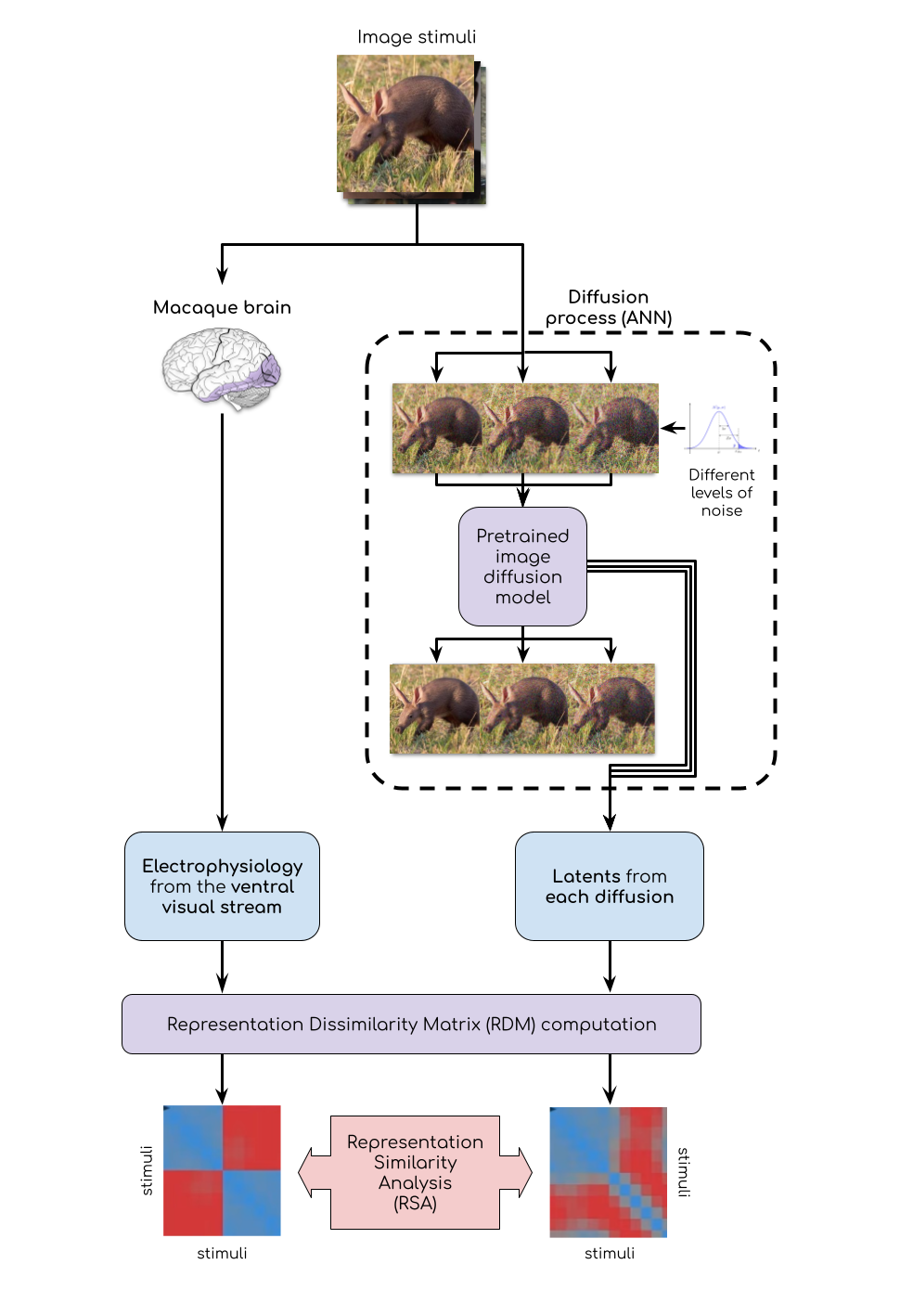
To answer our questions and test the validity of our hypothesis, we need to pass the same images through both a biological brain and a diffusion model and compare the internal representations. Our pipeline is built to be reproducible. It is fully open-source and can be accessed through the following link: https://github.com/ibrahimhabibeg/diffusion-brain-alignment.
2.1 The Neural Recordings and the Diffusion Model
To conduct our study, we utilized the THINGS Ventral-stream Spiking Dataset, TVSD (Papale and Roelfsema 2024), which contains electrophysiological recordings from V1, V4, and IT in two macaques in response to nearly 22k images from the THINGS image database (Hebart and Stoinski 2019; Hebart et al. 2019). The recordings in the TVSD would serve as the internal representations for the biological brain.
To generate the internal representations for the diffusion models, we need to pass the same images through the denoiser of a diffusion model. We decided to use the widely popular Stable Diffusion v1.5 model (Rombach et al. 2022) due to (1) its small size allowing inference without the need for high-end GPUs (2) its availability on HuggingFace making it easy to use through the Diffusers library (Platen et al. 2022), and (3) its usage of the U-Net architecture (Ronneberger et al. 2015) for the denoiser network, which simplifies the extraction of the model’s internal representations.
To decrease the computational burden of our analysis, we used a subset of the full THINGS dataset containing 1,854 images. To maintain diversity, this subset was created using only one image from each category in the original dataset and dropping all the other images. All the images were resized to 512x512 before passing them through the VAE of a pretrained Stable Diffusion v1.5 model to obtain their latent representations. Noise was added to the latent representation using the DDIM scheduler (Song et al. 2022) and 21 different values for the timestep. For clarity, we will refer to these timesteps as normalized noise levels ranging from 0.0 to 1.0. For example, a noise level of 0.99 means a high ratio of the latent being noise (almost pure Gaussian noise), while 0.01 represents a small ratio of the latent being noise (almost pure image information). The noised latents were then passed through the U-Net denoiser, and the representations were extracted from the bottleneck. These were then spatially averaged to produce a flat, 1280-dimensional representational vector for each image-timestep pair.
2.2 Representational Similarity Analysis
To quantify the similarity between the representations of the diffusion model and the recordings from the macaques, we used Representational Similarity Analysis (RSA) (Kriegeskorte 2008). The RSA approach is composed of two stages. First, we compute the representational dissimilarity matrix (RDM) to estimate the distance between the representations of each pair of images in the dataset. We compute these RDMs independently for every macaque brain region, as well as for every noise timestep in the diffusion model. In the second stage, we compare one of the artificial RDMs with one of the macaque RDMs and compute a score for the similarity of the two RDMs. The higher that score, the more similar those representations are.
We used the correlation distance to compute values in the RDM (i.e., calculate the dissimilarity between two representations), and we computed the RSA final scores using Spearman’s rho. Implementations of these algorithms can be found in the rsatoolbox Python library (Bosch et al. 2025). The toolbox is built to run on a CPU, and our analysis involved computing the RSA scores thousands of times. Therefore, we reimplemented these algorithms in PyTorch for GPU acceleration, and these implementations can be found in the project’s GitHub repository.
2.3 Performed Tests
Our first question was concerned with determining if there was any similarity between the representations of the diffusion model and the recordings from the macaque. To test this, we decided to follow the permutation-based statistical significance test described in Kriegeskorte (2008). The null hypothesis, \(H_0\), is that the two RDMs are unrelated. To perform this test, we randomly permute the rows and columns of one of the RDMs and compute the RSA score. We repeat this process a large number of times to generate a null distribution. The \(p\)-value is then calculated as the proportion of RSA scores in the null distribution that are greater than or equal to the observed RSA score. We reject \(H_0\) if the \(p\)-value is smaller than a predetermined significance level, \(\alpha\), where \(\alpha = 0.01\).
To establish the relationship between the similarity of the representation with respect to the noise level and the brain regions, we compute the RSA score for each combination of 21 different timesteps with each of the three brain regions. We also perform subsampling bootstrap to compute confidence intervals for each combination. Subsampling is performed by randomly sampling without replacement 80% of the stimuli and computing the RSA score 1,000 times. We use the generated scores to compute the 95% confidence interval for each combination.
To contextualize and better interpret our RSA scores, we computed the RSA scores between the two macaque brains for each brain region. This is based on our assumption that the diffusion model can not be more similar to one macaque than another macaque. Thus, these values were used to give us a sense of an upper bound for the similarity.
3 Results
In this section, we present our findings. First, we determine if there is a statistically significant relationship between the representations of the diffusion model and the recordings from the macaque brains. Then, we explore how this relationship varies across different noise levels and brain regions. Finally, we explore the RDMs.
3.1 Statistical Significance of Alignment
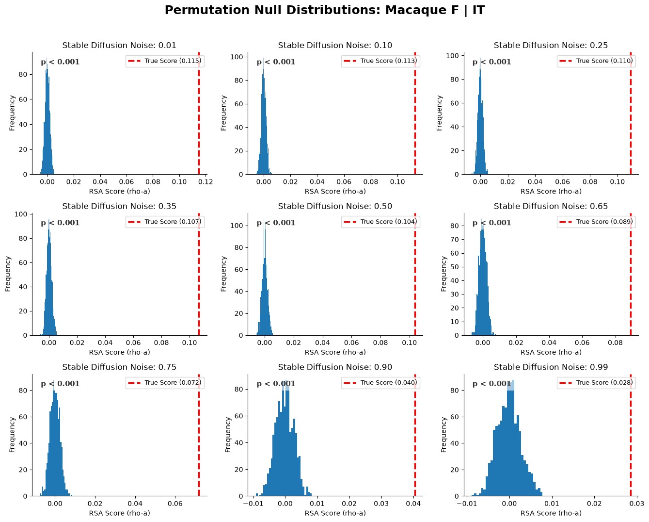
We begin our analysis by performing the permutation test described in Section 2.3. Figure 2 displays the results of the statistical test for 9 different timesteps compared with the IT region in the ventral visual stream of one of the macaques (monkey F). In this figure, we can observe that for all the tested timesteps the \(p\)-value is smaller than \(\alpha=0.01\), and as such we reject the null hypothesis and conclude that there is a relationship between the representations of the diffusion model and those of the tested regions in the macaque brains. We performed this test for a total of 21 timesteps, 3 brain regions, and 2 macaques, and all of them yielded the same results.
This answers our first research question and proves the validity of our initial hypothesis.
3.2 RSA Across the Noise Levels and Brain Regions
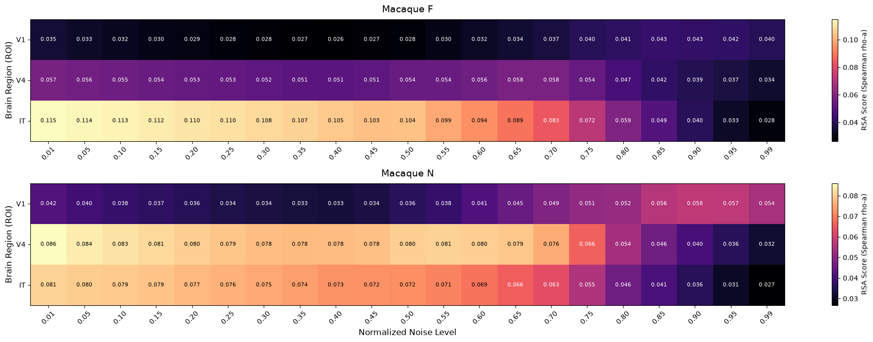
To determine how the alignment between the diffusion model and the macaque brains varies with noise levels and brain regions, we computed the RSA score for each combination of 21 different timesteps with each of the three brain regions for both macaques. Figure 3 displays the RSA scores for all the combinations. We observe that across both macaques, the alignment between the diffusion model representations and the IT and V4 regions is generally higher for less noisy representations. We also notice that the scores are lowest for the V1 region compared to the IT and V4 regions.
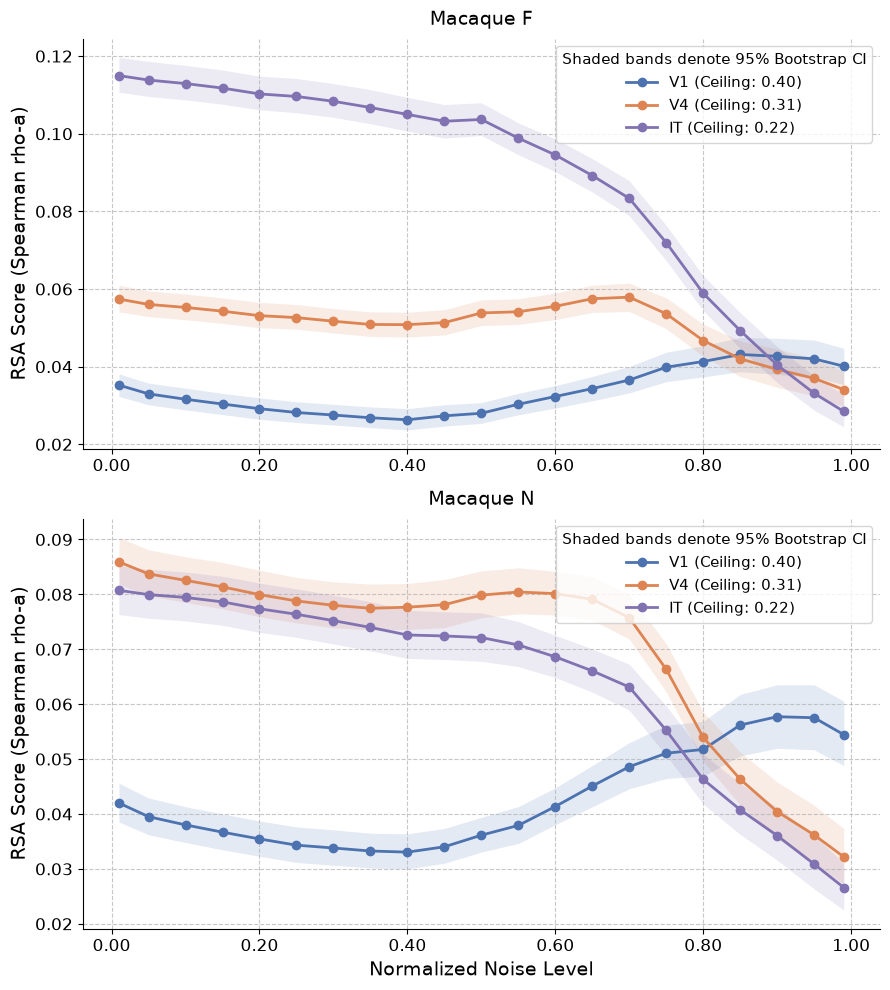
As discussed in Section 2.3, we performed subsampling bootstrap to compute confidence intervals for each combination to determine if the observed differences across timesteps are random or not. Figure 4 shows the mean RSA score across the bootstraps, and the shaded region shows the 95% confidence interval for each combination. This gives us more confidence believing that the alignment for the IT and V4 regions is higher when less noise is present.
Notably, this contradicts our earlier hypothesis. While we expected the similarity with the IT region to peak at more noisy timesteps, the results indicate the opposite. When the diffusion model sees the image more clearly, it is able to generate representations that are more aligned with the representations found in the macaque IT region. Our earlier thoughts were that at earlier timesteps (noisier inputs), the diffusion model is still putting in more effort to figure out the overall content of the image. At this stage it will be more focused on figuring out whether the image shows a dog or a cat rather than polishing tiny details in the animal’s fur, for example. We thought that these computations more closely resemble the higher-level processing of the IT region. The data, however, oppose our expectations, and we leave further discussion for possible reasons to Section 4.
The data here contradict our initial hypothesis, and we find that for the IT and V4 regions, the alignment increases at later stages of the diffusion process where the image is clearer to the model. For V1, the pattern was not as clear, but once again the data was against our hypothesis, and we saw a small peak in similarity at earlier timesteps.
3.3 Exploring the RDMs
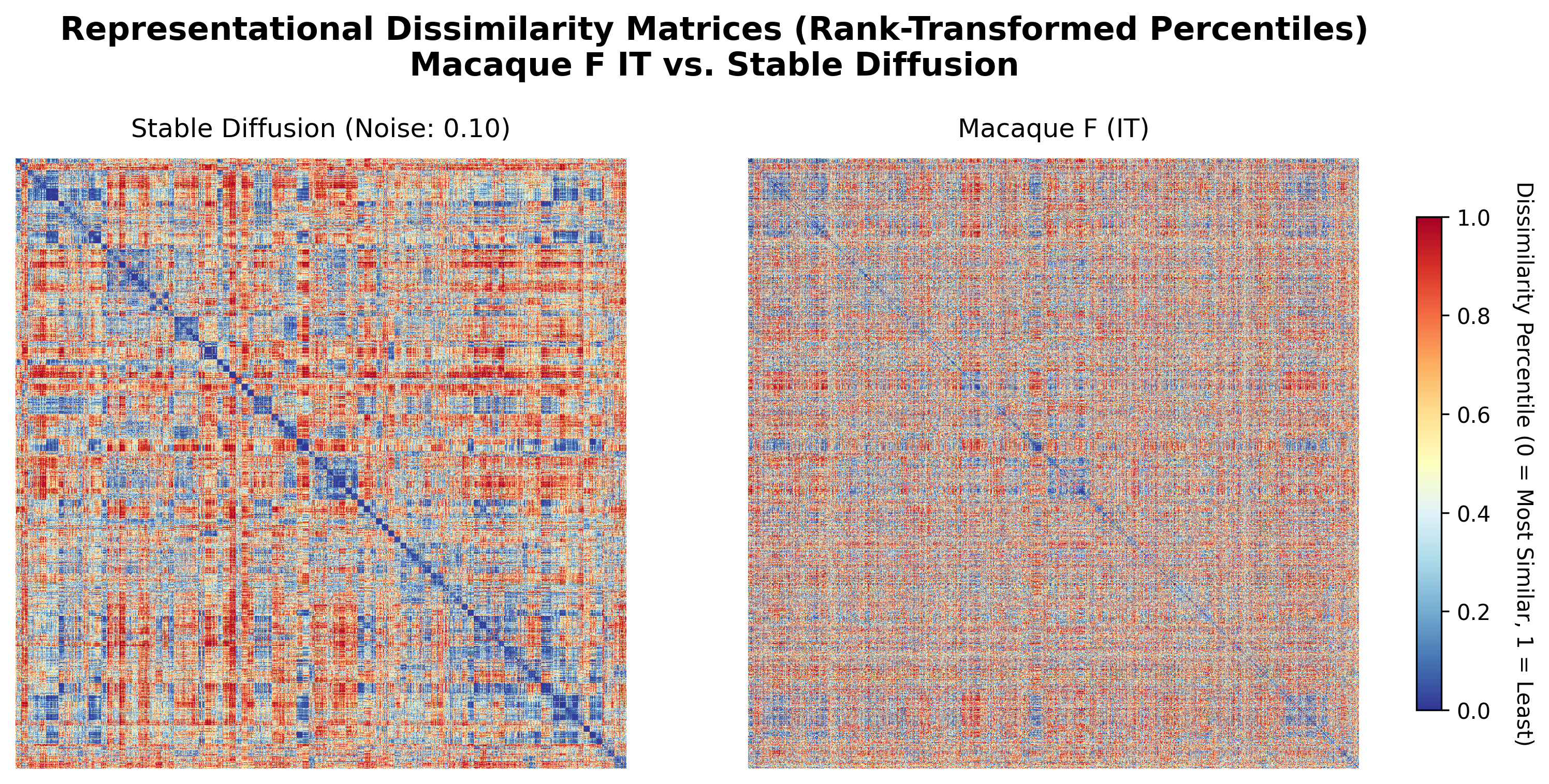
Another useful method of understanding what the networks are doing is to visualize the RDMs themselves. If the RDMs were plotted without any sense of ordering for the rows and columns, we would expect the matrix to look like TV static, since we would expect the pairwise distance between any two random images to be roughly the same. Since the THINGS dataset provides us with a category for each image, we can use them to order the rows and columns of the RDM in a way that allows us to visually inspect it.
Figure 5 displays a heatmap of the RDM for the IT region in Macaque F and that of Stable Diffusion at a 0.1 noise level. To generate these figures, we did not use the one-sample-per-category subset that we mentioned earlier and instead used a subset containing 100 different categories and 12 sample stimuli from each category. Stimuli coming from the same category were lined up next to each other, and the categories themselves were ordered so that conceptually similar items were grouped together. If the network at hand truly understands the semantics of the images, we should expect its RDM to have some block-like structure. This is because images of the same category, which are lined up next to each other, should have similar representations and should have a lower dissimilarity compared with the dissimilarity of one image with one outside the category. This means that we should expect the diagonal to be full of 12x12 squares of low dissimilarity value. Since the ordering of the categories is not random, we should also see some bigger squares which have the same color. If we found the RDM to look totally random with a lack of “squares”, then the representations of the network do not encode the semantics of the given stimuli.
Looking at Figure 5, we can see that the RDM of the diffusion model clearly exhibits the block-like structure we expected. Moving across the diagonal, we see the crisp, dark blue squares indicating the model’s ability to map images of the same category to similar representations. We also see some bigger blue squares along the diagonal, which is due to the model assigning similar categories similar representations. Moving to the RDM of the IT region in the macaque, we find a totally different story. The matrix looks much more random, and we can no longer see the squares which were clear in the other RDMs. For the V4 and V1 regions, the RDMs were even worse.
4 Open Questions and Future Directions
4.1 Changing the Biological Brain
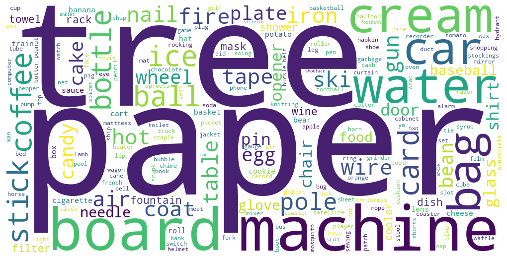
One surprising discovery was the lack of the expected block-like structure in the RDMs created from monkeys’ neural recordings (Figure 5). This raises the question of whether monkeys are the right subject to use in this comparison. Figure 6 shows a word cloud of the categories of the images contained in the dataset. We see that the images contain “things” that humans are familiar with (e.g., car, glove, cake, coffee), but a monkey would not be expected to understand their meaning or purpose. This could be the reason why the RDMs were noisy. Future work could investigate the validity of this hypothesis.
Another surprising discovery was the increase in alignment with the IT region as the images became less noisy, which contradicted our initial hypothesis. We know that at earlier timesteps diffusion models are putting in more effort to “imagine” what the image should be and deciding how to shape and manipulate the Gaussian noise to transform it into a clear visual. The lack of alignment of those stages with the IT could indicate that we are looking into the wrong regions of the brain. It could be that other regions are more responsible for this form of imagery. It is also possible that we are doing the wrong test and that we should be looking for brain representations while subjects are performing visual imagery rather than visual perception.
One approach that might help both lines of discovery is moving from the electrophysiological macaque data to human fMRI data. This helps the first line of discovery because it gives us representation of subjects who actually understand the meaning of the images. It also helps the second line because fMRI data contains recordings of the full brain, allowing us to look for peaks in similarity with regions outside the visual ventral stream. Datasets containing fMRI recordings of humans while viewing images are becoming increasingly popular. One example is Zerbe et al. (2026) which contains recordings for 5 subjects viewing over 25k images.
4.2 Disentangling Representations from the Architectural Bias
Eagle-eyed readers would notice in Figure 2 that even at a noise level of 0.99, not only was the \(p\)-value below the threshold, but it was actually at the lowest possible value as indicated by the fact that the true RSA score (red line) falls entirely outside the null distribution (blue bars). These results are consistent across the three regions and the two macaques. This was such a surprise that we tried performing the same test using Gaussian noise as input to ensure that our code is correct, and the scores failed to reject the null hypothesis as expected. We have two hypotheses for why this might be occurring. The first is due to the fact that we are using a latent diffusion model where noise is added to the highly compressed latent representation extracted by the VAE rather than added directly to the image as in pixel space diffusion models. It could be the case that the VAE is doing an incredible job at keeping the signal when compressing the image. Thus, even when a huge amount of noise is added, there is still enough information left for the denoiser network to use. Another hypothesis could be that the U-Net is just a merciless signal hunter that was able to extract the very faint signal from the noisy latents.
This also brings another question to our mind. How much of the alignment is due to the training? We know that architectures like the U-Net, which rely on convolutions, have very strong inductive biases for vision tasks. It is possible that the alignment is just due to the use of a strong architecture and that the training does not help much. Future work could investigate why a relationship was found at high noise levels and could study the effect of training on the similarity. A possible next step is performing the same analysis using the same network, but with random weights to help us study the effect of training.
4.3 Effect of Model Architecture on Alignment with the Brain
Another possible line of future work is looking into different frameworks of diffusion and looking into different architectures. While we saw strong resilience to noise in latent diffusion models, pixel-space diffusion models could be less tolerant to added noise because noise is directly added to the image instead of the highly compressed representations. Moreover, while the vast majority of diffusion models use networks to parameterize the noise added to the image, other approaches include directly parameterizing the image or a combination of the image and the noise (Li and He 2026). Future work could investigate if directly predicting the image makes the model more similar to the brain.
5 Conclusion
In this work, we explored whether Stable Diffusion encodes images similarly to the primate visual stream and for which timesteps the similarity peaks. We found statistically significant evidence that a non-zero relationship exists between the diffusion model’s representations and the macaque’s representations. For the IT region, this similarity contradicted our initial expectations and peaked at the later timesteps. This surprise, along with others, paves the way for future research to further explore this phenomenon and gain a better understanding of the connection between diffusion models and the brain.
5.1 Limitations
Recordings from the brain are noisy, and repeating the same stimuli to the same subject can lead to different recordings. For the stimuli we used, we had only one recording per stimulus. Moreover, some channels could be faulty and have more noise in them than usual. In our analysis, however, all the channels from the electrophysiological recordings were used.
6 Acknowledgements
This project was developed during the NeuroAI course of the Neuromatch Academy 2026. We thank our project TA, Reza Rajabli, for his guidance and support throughout the project. We also thank our pod TA, Tshiangomba Kasonsa, for his help throughout the academy. We are grateful to the Neuromatch Academy for providing this opportunity to learn and collaborate on this project.
References
Baranchuk, Dmitry, Ivan Rubachev, Andrey Voynov, Valentin Khrulkov, and Artem Babenko. 2022. Label-Efficient Semantic Segmentation with Diffusion Models. arXiv. https://doi.org/10.48550/arXiv.2112.03126.
Bosch, Jasper JF van den, Tal Golan, Benjamin Peters, et al. 2025. A Python Toolbox for Representational Similarity Analysis. https://doi.org/10.1101/2025.05.22.655542.
Hebart, Martin N., Adam H. Dickter, Alexis Kidder, et al. 2019. “THINGS: A Database of 1,854 Object Concepts and More Than 26,000 Naturalistic Object Images.” PLOS ONE 14 (10): e0223792. https://doi.org/10.1371/journal.pone.0223792.
Hebart, Martin N, and Laura Mai Stoinski. 2019. THINGS Object Concept and Object Image Database. https://doi.org/10.17605/OSF.IO/JUM2F.
Huh, Minyoung, Brian Cheung, Tongzhou Wang, and Phillip Isola. 2024. The Platonic Representation Hypothesis. arXiv. https://doi.org/10.48550/arXiv.2405.07987.
Kriegeskorte, Nikolaus. 2008. “Representational Similarity Analysis – Connecting the Branches of Systems Neuroscience.” Frontiers in Systems Neuroscience, ahead of print. https://doi.org/10.3389/neuro.06.004.2008.
Li, Tianhong, and Kaiming He. 2026. Back to Basics: Let Denoising Generative Models Denoise. arXiv. https://doi.org/10.48550/arXiv.2511.13720.
Mukhopadhyay, Soumik, Matthew Gwilliam, Vatsal Agarwal, et al. 2023. Diffusion Models Beat GANs on Image Classification. arXiv. https://doi.org/10.48550/arXiv.2307.08702.
Papale, Paolo, and Pieter Roelfsema. 2024. TVSD: THINGS Ventral-Stream Spiking Dataset. G-Node. https://doi.org/10.12751/G-NODE.HC7ZLV.
Platen, Patrick von, Suraj Patil, Anton Lozhkov, et al. 2022. Diffusers: State-of-the-Art Diffusion Models. GitHub. https://github.com/huggingface/diffusers.
Rombach, Robin, Andreas Blattmann, Dominik Lorenz, Patrick Esser, and Bjorn Ommer. 2022. “High-Resolution Image Synthesis with Latent Diffusion Models.” 2022 IEEE/CVF Conference on Computer Vision and Pattern Recognition (CVPR) (New Orleans, LA, USA), June, 10674–85. https://doi.org/10.1109/CVPR52688.2022.01042.
Rosenblatt, F. 1958. “The Perceptron: A Probabilistic Model for Information Storage and Organization in the Brain.” Psychological Review 65 (6): 386–408. https://doi.org/10.1037/h0042519.
Schrimpf, Martin, Jonas Kubilius, Ha Hong, et al. 2018. Brain-Score: Which Artificial Neural Network for Object Recognition Is Most Brain-Like? Neuroscience. https://doi.org/10.1101/407007.
Schrimpf, Martin, Jonas Kubilius, Michael J. Lee, N. Apurva Ratan Murty, Robert Ajemian, and James J. DiCarlo. 2020. “Integrative Benchmarking to Advance Neurally Mechanistic Models of Human Intelligence.” Neuron 108 (3): 413–23. https://doi.org/10.1016/j.neuron.2020.07.040.
Song, Jiaming, Chenlin Meng, and Stefano Ermon. 2022. Denoising Diffusion Implicit Models. arXiv. https://doi.org/10.48550/arXiv.2010.02502.
Yamins, Daniel, Ha Hong, Charles Cadieu, and James J DiCarlo. 2013. “Hierarchical Modular Optimization of Convolutional Networks Achieves Representations Similar to Macaque IT and Human Ventral Stream.” Advances in Neural Information Processing Systems 26. https://papers.nips.cc/paper_files/paper/2013/hash/9a1756fd0c741126d7bbd4b692ccbd91-Abstract.html.
Zador, Anthony, Sean Escola, Blake Richards, et al. 2023. “Catalyzing Next-Generation Artificial Intelligence Through NeuroAI.” Nature Communications 14 (1): 1597. https://doi.org/10.1038/s41467-023-37180-x.
Zerbe, Josefine, Johannes Roth, Maggie Mae Mell, Peer Herholz, Tomas Knapen, and Martin N. Hebart. 2026. LAION-fMRI: A Densely Sampled 7T-fMRI Dataset Providing Broad Coverage of Natural Image Diversity. https://www.visionsciences.org/talk-sessions?id=642.